Last year, when we got our article accepted by Nature, there was an interesting line in the acceptance email that stood out to us:
If you have not already done so, you may send potential cover suggestion file(s) to the production department […]. The file(s) should be sent within a week of receiving this email in order to be considered, and we cannot promise that your cover suggestion will be used, as competition is intense.
Besides being over the moon about the acceptance, we hadn’t really expected to be able to submit a cover. It also meant there was a very tight deadline to create this image. Thanks to a suggestion from our editor, we had a starting point in the form of one of our figures, which depicts the scattering event and the associated waveform of the gravitational wave.
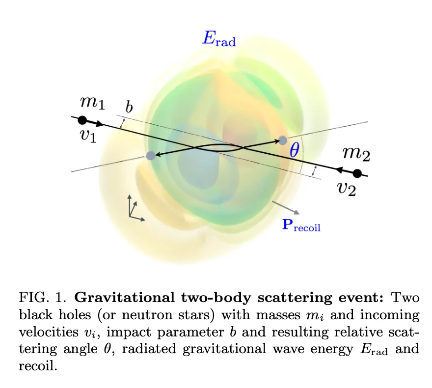
This figure was a still from a video created by a bachelor’s student and wasn’t very high-resolution or accurate 1. It’s a visualization of a formula that dates back to two pioneers in general relativity, Kovács and Thorne, from their paper The generation of gravitational waves. IV. Bremsstrahlung. (see eqs. 3.17-18).
From general relativity, we know that just like electromagnetic waves have two polarization states, so do gravitational waves. The difference is that electromagnetic waves are typically thought of as vertically or horizontally polarizated, while for gravitational waves are a bit more complicated — the two states are “cross” and “plus”.
Writing it down as one optimized numba function of , , , (the four spacetime coordinates), and (the masses of both black holes/compact objects), (the impact parameter), and (the relative Lorentz factor), it’s about 400 lines of python, which you can find available for download With some quick python scripting and rough plotting with matplotlib, I had some ranges I thought would look good.
After some experimentation with different pieces of software, I settled on ParaView. ParaView is a phenomenal piece of software for visualizing large amounts of scientific data up to the supercomputer scale. It can slices up and transform your data however you want.
Unfortunately, ParaView doesn’t natively support reading in arbitrary numpy arrays. I recommend the VTK format. You can convert it as follows:
import numpy as np
import vtk
from tqdm import tqdm
from vtkmodules.util import numpy_support

frames = np.load("waveform_cross.npy")

for i, frame in tqdm(enumerate(frames)):
    image_data = vtk.vtkImageData()
    image_data.SetDimensions(100, 100, 100)
    vtk_array = numpy_support.numpy_to_vtk(num_array=frame.ravel(), deep=True, array_type=vtk.VTK_FLOAT)
    vtk_array.SetName("cross_strain")
    image_data.GetPointData().AddArray(vtk_array)
    image_data.GetPointData().SetScalars(vtk_array)
    writer = vtk.vtkXMLImageDataWriter()
    writer.SetFileName(f"waveform/strain_waveform_plus_{i:03d}.vti")
    writer.SetInputData(image_data)
    writer.Write()
Once you’ve done that, you can import the contents of the waveform folder as a series and it’ll play back within ParaView as a movie, frame by frame (your computer might have a little trouble doing this quickly).
When you import the data into ParaView, it will not look good. That’s because it’s three-dimensional data, so when represented on a two-dimensional screen, parts of it will inherently block other parts. The trick is to find a visualization method that will have a large amount of transparency so that we can really see all of the object, but opaque enough so that any one part doesn’t feel nebulous or vague.
The trick I settled on was the equivalent of plotting contour lines in three dimensions. This is something that ParaView does beautifully because it can interpolate your data. I generated it originally with a 100 x 100 x 100 grid, which is very rough for a visualization of this quality, but ParaView makes it look beautiful and smooth.
The way I implemented this contour plot is the only bit that took an artistic flair. I implemented it by taking the rainbow color scheme and adjusting the opacity curve to look like a comb function (slightly smoothed, of course). This made certain colors particular prominent. It is slightly misleading in the sense that each new shell isn’t a new wavefront, even though it looks like it.